Project 1 - Quantum Circuit Simulator
Quantum Circuit Simulator
Submit to Autograder by 11:55pm Tuesday 2/10
Learning Objectives
After successfully completing this project, students will have a thorough understanding of how quantum states and circuits are represented, and how computation is done at an abstract level.
Introduction
In this project, you will write a simulator for a simple quantum computer, the Little Quantum Computer 3000 (LQ3K). This simulator supports constructing a quantum circuit using a small set of gates, calculating the unitary representation of that circuit, and simulating the result of running the circuit with a given state vector by either returning the resulting state vector (deterministic) or performing a measurement on all bits and returning the measured value (probabilistic). This is effectively a (very) scaled down version of the Qiskit library, which you will use in the remainder of the course.
Project Details
The simulator is implemented as a Python class. We have provided method stubs for you to complete. You are welcome to add additional methods or member variables as you wish, but you must not change the method declarations provided.
These are the following gates supported by the LQ3K simulator:
- X
- Y
- Z
- S
- S dag (complex conjugate of S)
- T
- T dag (complex conjugate of T)
- Hadamard (H)
- SWAP
- Controlled Not (CX)
The LQ3K does NOT support arbitrary measurements. The only way to measure a circuit is to run simulate_run() on an object after composing the circuit. This will automatically measure every qubit in the circuit at the end of computation and return the results.
The simulate_run() function takes in a numpy.array as input. The simulator follows the same ordering conventions as presented in lecture, i.e. index N holds the probability amplitude of \(\ket N\). For example, in a 2-qubit system the state \(\ket{q_1q_0} = a\ket{00} + b\ket{01} + c\ket{10} + d\ket{11}\) is represented by the numpy array [a, b, c, d].
Testing
You must provide a set of test functions written in tests_p1.py to the autograder. You must use the Unittest model discussed in lab. Your tests will be graded on whether they cause assertion failures when run on buggy solutions, but do not cause assertion failures on correct implementations.
Error Handling
Your implementations for simulate_run() must check that the provided state vector is valid, i.e. that the norm is approximately 1. Note that due to floating-point rounding, a valid vector may have a calculated norm slightly off (e.g. something like 0.99999987). You should use numpy.allclose to verify that the norm is sufficiently close to 1 (the default tolerance of 1e-08 is fine). If any invalid input is provided, your code must raise an LQ3K.InvalidStateVector exception.
Restrictions
Complete all function methods in p1.py and all method tests in tests_p1.py. The only packages you may import are numpy, random, typing, and unittest. The autograder is running Python 3.10.12 and NumPy version 2.2.2. It is recommended that you use a virtual environment and install dependencies from the provided requirements.txt. You only need to do the below once:
$ python -m venv .venv
$ source .venv/bin/activate
$ pip install -r requirements.txt
and then this whenever you start a new terminal instance:
$ source .venv/bin/activate
Submission and Grading
Submit p1.py and tests_p1.py to the autograder using the direct link at the top of this page. Your final grade is out of 100 points.
We will grade your code on functional correctness. As a reminder, you may not share any part of your code with others in a way that can be copied. You are encouraged, however, to discuss the project with each other and help each other with problems you may encounter. You will get feedback on your total score, but you will not have access to what the private test cases are checking for.
Efficiency is not graded, but your code must complete in a reasonable amount of time. Note that for general quantum circuits, simulation takes an exponential amount of time. We will only grade your code on circuits containing up to 5 qubits.
The output of simulate_run() is generally non-deterministic but should follow a precise distribution for a given circuit. We will grade this function by running it a circuit 1000 times and verifying that it matches the theoretical distribution within 11.7% (this provides a Z-score of 3.719, meaning a correct implementation should fail less than once in 10,000 runs).
Appendix
You are free to implement this simulator however you see fit. However, we recommend modeling each circuit as a unitary matrix using numpy.array objects. Each addition of a gate should update this matrix accordingly, and passing a given state vector through the circuit can be implemented by multiplying the matrix representation with the state vector. See the course reference for a brief overview on how to deal with matrices and vectors in Python using NumPy. Below is a brief description on how to approach each section of the project using this strategy.
Single qubit gates
Applying a single qubit gate to a multi-qubit circuit is equivalent to applying the Identity operation to every remaining qubit. The overall operation can be described as an appropriate Kronecker (i.e. tensor) product between several instances of the Identity matrix and the 2x2 matrix representing the single qubit gate.
SWAP
Swap is easier to implement if the qubits being swapped are adjacent. In that case, the full operation can be described by Kronecker products between Identity matrices and the 4x4 matrix representing the SWAP operation discussed in lecture.
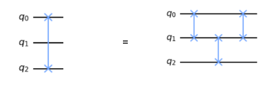
Swapping non-adjacent qubits can be implemented through multiple swaps of adjacent qubits. E.g. swapping [0,2] can be done by swapping [0,1], then [1,2], then [0,1] again.
CNOT
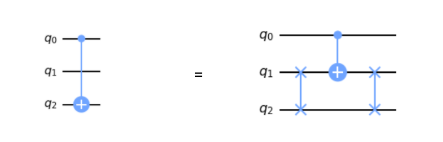
As with SWAP, CNOT is easiest when the bits are adjacent (allowing for a simple Kronecker products between Identity matrices and the 4x4 CNOT matrix described in lecture). For non-adjacent qubits, SWAP can be used to move one of the qubits to be adjacent, and then swapped back after the CNOT is applied.
Applying multiple gates
Applying multiple gates in sequence is equivalent to performing a matrix multiplication between the matrices representing those gates.
Simulating Circuit
When simulating measurement of your circuit, you must randomly choose one of the possible outcomes, waited by a set of calculated probabilities. You may find the random.choices function helpful here. If outcomes is a list holding the possible outcomes, and probabilities is a list such that probabilities[i] is the probability of measuring outcomes[i], then the following statement will select one of the outcomes with the appropriate probability (the function returns a list, which is why you must access [0] at the end to read the actual outcome):
random.choices(outcomes, probabilities)[0]
Remember that when testing this function, you should allow for a slight deviation from expected values, since the output is nondeterministic. Allowing a 10% deviation should be plenty, while still catching meaningful bugs.